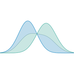
f-Divergence

Chapter 14: Information Theory. In the chapter mind map this icon labels JS-Divergence, f-Divergence, Wasserstein. The discussion below is excerpted and lightly edited from § Definition: KL Divergence in Mathematics for AI and Machine Learning.

For two probability distributions over the same space, the Kullback–Leibler (KL) divergence is defined as follows. For discrete distributions with probability mass functions $p(x)$ and $q(x)$, and for continuous distributions with probability density functions $f(x)$ and $g(x)$:

KL divergence measures the expected extra information (or "surprise") when using distribution $q$ to encode events that actually follow distribution $p$, or equivalently, the amount of information lost when using $q$ to replace $p$. In machine learning, $p$ typically represents the true data distribution and $q$ represents the model distribution. Minimizing $D_{\mathrm{KL}}(p || q)$ makes the model $q$ match the data distribution $p$.

Following standard convention, we use lowercase $p$ and $q$ as generic notation for probability distributions (PMFs for discrete, PDFs for continuous). When the context is clear, we write $D_{\mathrm{KL}}(p || q)$ for both cases.

the book figure shows the setting the definition requires: $P$ and $Q$ live on the same sample space $\{1, \ldots, m\}$, so $p(x)/q(x)$ is defined at every outcome. The divergence accumulates where the two disagree, weighted by $p(x)$, and vanishes where the bars coincide.