GPTQ Hessian

Chapter 10: Matrix Block Partitioning. In the chapter mind map this icon labels Hessian Block Structure & GPTQ Block-wise Quantization. The discussion below is excerpted and lightly edited from § GPTQ: Block Structure in Quantization in Mathematics for AI and Machine Learning.

GPTQ (Frantar et al., 2023) is a post-training quantization method that rounds the weights of a trained model to a few bits (e.g., 4) while compensating the rounding error with second-order information. It quantizes one linear layer at a time and treats the layers as independent, which amounts to keeping only the diagonal (per-layer) blocks of the network's Hessian. Within a layer, block structure then makes the second-order method both exact and cheap.

For a linear layer with weight matrix $W \in \mathbb{R}^{d_{\text{out}} \times d_{\text{in}}}$ and calibration inputs $X \in \mathbb{R}^{d_{\text{in}} \times n}$ ($n$ tokens), GPTQ seeks a quantized $\hat{W}$ that minimizes the layer's reconstruction error:

In practice a small damping term is added, $H = 2XX^\top + \lambda I$, so that $H$ is positive definite. Writing $\mathbf w_i^\top$ for row $i$ of $W$, the objective splits into a sum over rows, $\sum_i (\mathbf w_i - \hat{\mathbf w}_i)^\top XX^\top (\mathbf w_i - \hat{\mathbf w}_i)$: every row has the same Hessian $H$.

Stack the rows of $W$ one under another into a single vector of length $d_{\text{out}} d_{\text{in}}$. The Hessian of the objective with respect to this vector is the Kronecker product (@eq:kronecker-product-definition)

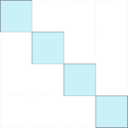
a block-diagonal matrix with $d_{\text{out}}$ identical $d_{\text{in}} \times d_{\text{in}}$ blocks. For $d_{\text{out}} = d_{\text{in}} = 4096$, $H_{\text{layer}}$ is a $16{,}777{,}216 \times 16{,}777{,}216$ matrix, yet it is determined by the single $4096 \times 4096$ matrix $H$. The block structure is exact, not an approximation: the rows decouple, and one Cholesky factorization of $H^{-1}$, costing $O(d_{\text{in}}^3)$, serves every row.

GPTQ quantizes the columns of $W$ in order $j = 0, 1, \ldots, d_{\text{in}} - 1$. After rounding column $j$, it corrects the columns not yet quantized to absorb the error (the Optimal Brain Surgeon update; see the matrix chapter). Let $U$ be the upper triangular Cholesky factor of $H^{-1}$, so $H^{-1} = U^\top U$. The columns are processed in blocks of $B$ columns (typically $B = 128$). For each column $j$ of the current block $\mathcal B$,