Joint and Marginal Distributions

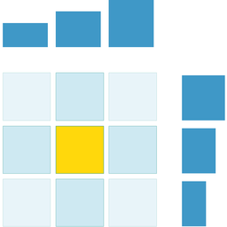
Chapter 13: Probability and Random Variables. In the chapter mind map this icon labels Joint, Marginal, & Conditional Probabilities. The discussion below is excerpted and lightly edited from § Marginal Probabilities in Mathematics for AI and Machine Learning.

Given a joint distribution, we often care about one variable alone. The marginal distribution of $X$ is obtained by summing (or integrating) the joint over all values of $Y$: we forget $Y$ by adding up every way it could have happened. The name comes from tables. Write the joint PMF as a table with one column per value of $X$ and one row per value of $Y$; the column sums, written in the bottom margin, are $P(X=x)$, and the row sums, written in the right margin, are $P(Y=y)$.

the book figure shows this for a joint PMF on the grid $\{0,\dots,8\}^2$. Summing each column of the joint surface projects it onto the wall behind it and gives $P(X=x)$; summing each row projects it onto the side wall and gives $P(Y=y)$ (dashed grey arrows). No probability is lost: each marginal sums to 1 because the joint does.