Detailed Balance

Chapter 21: Fokker-Planck and Distribution Dynamics. In the chapter mind map this icon labels Stationary Distributions and Detailed Balance. The discussion below is excerpted and lightly edited from § Stationary Distributions and Detailed Balance in Mathematics for AI and Machine Learning.

The target $p$ is a stationary solution: since $p \nabla \log p = \nabla p$, the drift term $\nabla \cdot (p \nabla \log p) = \nabla^2 p$ cancels the diffusion term, so at $p_t = p$

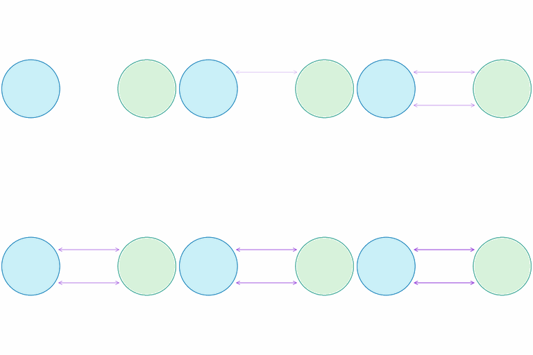
In fact the probability current $\mathbf{J} = p \nabla \log p - \nabla p$ vanishes identically at $p$, the detailed balance condition. Under appropriate conditions (ergodicity, irreducibility) this stationary solution is unique and every initial density $p_0$ converges to it as $t \to \infty$, at a rate set by the geometry of $p$. This is the distributional reason why Langevin dynamics samples correctly. the book figure shows it numerically: $D_{\mathrm{KL}}(p_t \| p)$ decreases monotonically (top), and snapshots of $p_t$ approach the target (bottom).