Fokker-Planck Equation
Chapter 21: Fokker-Planck and Distribution Dynamics — Fokker-Planck Equation
From the book
Chapter 21: Fokker-Planck and Distribution Dynamics. In the chapter mind map this icon labels Fokker-Planck Equation: Drift & Diffusion Terms. The discussion below is excerpted and lightly edited from § Numerical Methods for Fokker-Planck Equations in Mathematics for AI and Machine Learning.
In low dimensions the Fokker–Planck equation can be solved directly, by finite difference methods on a grid or by spectral methods that expand $p_t$ in basis functions such as Hermite polynomials. Both need a number of unknowns exponential in the dimension $d$ (a grid with $N$ points per axis has $N^d$ points, the curse of dimensionality), which rules them out for images. Diffusion models therefore never represent $p_t$: they learn the score and simulate the SDE or ODE, which solves the Fokker–Planck equation implicitly through samples. The equation remains the tool for analysis, design and convergence proofs.
What this drawing shows
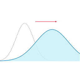
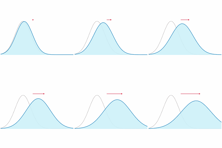
What you see. Shows $p(x,t)$ evolving under Fokker--Planck dynamics: gray dashed $p_0$ fixed while blue density drifts right and spreads (diffusion); red arrow tracks drift.
In the mind map. Chapter 21 — Fokker-Planck Equation: Drift & Diffusion Terms. See From the book above for definitions, figures, and worked examples.
Where to read next
Read the full definitions, figures, and worked examples in Chapter 21: Fokker-Planck and Distribution Dynamics — see the mind-map node Fokker-Planck Equation: Drift & Diffusion Terms.