Reverse Fokker-Planck

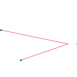
Chapter 21: Fokker-Planck and Distribution Dynamics. In the chapter mind map this icon labels Reverse-Time Fokker-Planck. The discussion below is excerpted and lightly edited from § Reverse-Time Fokker-Planck in Mathematics for AI and Machine Learning.

Reversing time in the forward SDE yields a reverse-time Fokker–Planck equation. For the reverse SDE (the matrix chapter):

the corresponding Fokker–Planck equation (taking into account the reversed direction of time $dt < 0$) is:

Expanding the drift term using $\nabla \log p_t = \frac{\nabla p_t}{p_t}$ gives $-\nabla \cdot (\mathbf{f} p_t) + \nabla \cdot (\mathbf{D}\nabla p_t)$. Combined with the negative diffusion term $-\frac{1}{2}\nabla \cdot (\mathbf{D}\nabla p_t)$, this recovers: confirming that the reverse SDE exactly matches the forward marginal distributions $p_t$.

The reverse equation involves the score $\nabla_{\mathbf{x}} \log p_t$ of the very densities it is supposed to produce, so it cannot be solved from $\mathbf{f}$ and $\mathbf{G}$ alone: the forward process is well-posed, the reverse one is not until the score is known. This is why diffusion models first learn $\mathbf{s}_\theta(\mathbf{x}, t) \approx \nabla_{\mathbf{x}} \log p_t$ by denoising score matching (the matrix chapter) from forward-process samples, and only then sample by running the reverse SDE or the probability flow ODE.

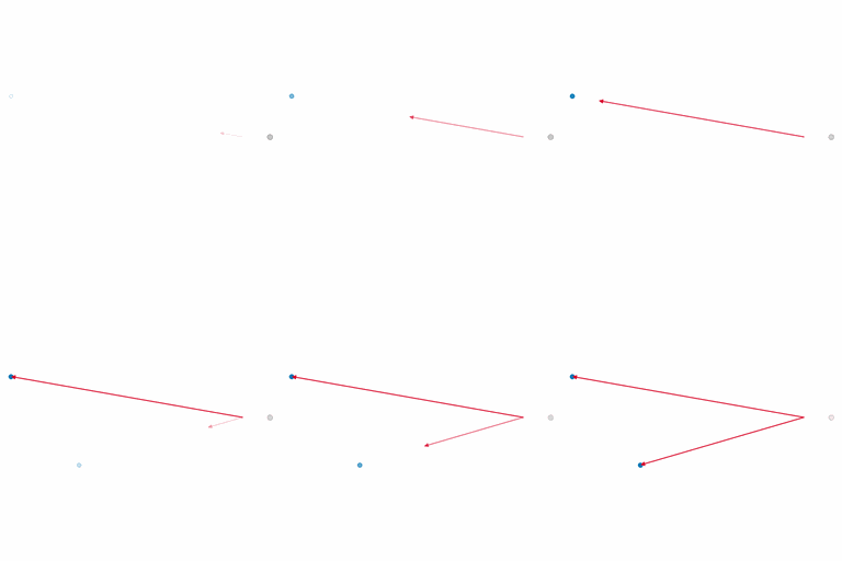
the book figure contrasts the two directions on a five-mode "star" distribution. Forward, the diffusive flux $-\nabla p_t$ spreads the modes into an unstructured cloud and destroys the information about where they were; backward, the score field $\nabla\log p_t$ points uphill, against the gradient of entropy, and carries the cloud back to the modes. Without the score the reverse process has nothing to tell it where the lost structure was, which is why score learning is necessary for generation by time reversal.